Location Set Covering Problem (LSCP) - Real World Facility Location Problem
geospatial
map
spatial optimization
Introduction
Location Set Covering Problem (LSCP) fall within a class of problems known as set covering problems. The set covering problem class is an NP-hard problem within the combinatorial optimization space. These problems typically aim at minimizing the number of sets within a space that cover all the demand within that space.
The Location Set Covering Problem is described by Toregas et al. (1971). There they show that emergency services must be placed according to a response time, since there is a allowable maximum service time for handling emergency activities. Therefore the LSCP model was proprosed whereby
the minimum number of facilities determined and locaten so that every demand area is covered within a predefined maximal service distance or time
(Church and Murray, 2018).
The general scenarios for this project can be stated as: store sites should supply the demand in this census tract considering the distance between the two sets of sites: demand points and candidate supply sites. Four fundamental facility location models are utilized to highlight varying outcomes dependent on objectives: LSCP (Location Set Covering Problem), MCLP (Maximal Coverage Location Problem), P-Median and P-Center.
Location Set Covering Problem (LSCP)
Location Set Covering is a problem realized by Toregas, et al. (1971). He figured out that emergency services must have placed according to a response time, since, there is a allowable maximum service time when it’s discussed how handle an emergency activity. Minimize the number of facilities needed and locate them so that every demand area is covered within a predefined maximal service distance or time. Since the model needs a distance cost matrix we should define some variables.
Maximal Coverage Location Problem (MCLP)
LSCP try to minimize the amount of facilities candidate sites in a maximum service standard but then arise another problem: the budget. Sometimes it requires many facilities sites to reach a complete coverage, and there are circumstances when the resources are not available and it’s plausible to know how much coverage we can reach using a exact number of facilities. MCLP class try to solve this problem:
Maximize the amount of demand covered within a maximal service distance or time standard by locating a fixed number of facilities self.
P-Center Problem
Hakimi (1964) introduced the absolute center problem to locate a police station or a hospital such that the maximum distance of the station to a set of communities connected by a highway system is minimized. Hakimi (1965) generalizes the absolute center problem to the p-center problem.
P-Median Problem
Hakimi (1965) proposed this model thinking about locating telephone switching centers. Then the objective was to minimize the total length of wire serving all customers while locating telephone witching centers, assuming that each customer would be connected by wire to the closest switching center. Locate a fixed number of facilities such that the resulting sum of travel distances is minimized
Dataset
Load dataset
For this project, we will solve mulitple real world facility location problems using a dataset describing an area of census tract 205, San Francisco.
The problem is composed by 4 dataset:
- network_distance is the calculus of distance between facility candidate sites calculated by ArcGIS Network Analyst Extension
- demand_points represents the demand points with some important features for the facility location problem like population
- facility_points represents the stores that are candidate facility sites
- study_area is the polygon of census tract 205.
network_distance = pd.read_csv(r"..\map\map_service_area\SF_network_distance_candidateStore_16_censusTract_205_new.csv")

demand_points = pd.read_csv(r"..\map_service_area\SF_demand_205_centroid_uniform_weight.csv", index_col=0)
demand_points_gdf = gpd.GeoDataFrame( demand_points,geometry=gpd.points_from_xy(demand_points.long, demand_points.lat),).sort_values(by=['NAME']).reset_index()

facility_points = pd.read_csv(r"..\map_service_area\SF_store_site_16_longlat.csv", index_col=0)
facility_points_gdf = gpd.GeoDataFrame( facility_points, geometry=gpd.points_from_xy(facility_points.long, facility_points.lat),).sort_values(by=['NAME']).reset_index()

study_area = gpd.read_file(r"..\map_service_area\ServiceAreas_4.shp").dissolve()
network distance
| distance | name | DestinationName | demand | |
|---|---|---|---|---|
| 0 | 671.573 | Store_1 | 6.07505e+07 | 6540 |
| 1 | 1333.71 | Store_1 | 6.07505e+07 | 3539 |
| 2 | 1656.19 | Store_1 | 6.07504e+07 | 4436 |
| 3 | 1783.01 | Store_1 | 6.07506e+07 | 231 |
| 4 | 1790.95 | Store_1 | 6.07505e+07 | 7787 |
demand points
| index | OBJECTID | ID | NAME | STATE_NAME | AREA | POP2000 | HOUSEHOLDS | HSE_UNITS | BUS_COUNT | long | lat | geometry | |
|---|---|---|---|---|---|---|---|---|---|---|---|---|---|
| 0 | 136 | 139 | 6075010100 | 6.07501e+07 | California | 0.29101 | 2879 | 1760 | 1944 | 538 | -122.411 | 37.8054 | POINT (-122.411302937 37.8053570610001) |
| 1 | 195 | 198 | 6075010200 | 6.07501e+07 | California | 0.19945 | 4288 | 2767 | 3044 | 256 | -122.422 | 37.8027 | POINT (-122.42182845 37.8026681890001) |
| 2 | 196 | 199 | 6075010300 | 6.07501e+07 | California | 0.1047 | 4092 | 2092 | 2327 | 78 | -122.415 | 37.8013 | POINT (-122.415180848 37.8012525410001) |
| 3 | 191 | 194 | 6075010400 | 6.07501e+07 | California | 0.13005 | 4859 | 2630 | 2899 | 209 | -122.408 | 37.8024 | POINT (-122.407959434 37.8023538830001) |
| 4 | 42 | 42 | 6075010500 | 6.07501e+07 | California | 0.26295 | 2217 | 1521 | 1843 | 925 | -122.4 | 37.7987 | POINT (-122.399951658 37.798735326) |
facility points
| index | OBJECTID | NAME | long | lat | geometry | |
|---|---|---|---|---|---|---|
| 0 | 1 | 1 | Store_1 | -122.51 | 37.7724 | POINT (-122.510018182 37.7723636370001) |
| 1 | 8 | 8 | Store_11 | -122.434 | 37.6554 | POINT (-122.433781818 37.6553636360001) |
| 2 | 9 | 9 | Store_12 | -122.439 | 37.7192 | POINT (-122.438981818 37.719236364) |
| 3 | 10 | 10 | Store_13 | -122.44 | 37.7454 | POINT (-122.440218181 37.7453818180001) |
| 4 | 11 | 11 | Store_14 | -122.422 | 37.743 | POINT (-122.421636364 37.7429636370001) |
polygon of census tract 205
| geometry | FacilityID | Name | FromBreak | ToBreak | FacilityOI | NAME_1 | Shape_Leng | Shape_Area | |
|---|---|---|---|---|---|---|---|---|---|
| 0 | POLYGON ((-122.45299324702856 37.638982033270395, -122.4541513019999 37.638532816000065, )) | 8 | Store_11 | 0 | 5000 | 8 | Store_11 | 0.287448 | 0.00333851 |

Data Preparation
Before running any analysis, we need to ensure that our data is well-structured and ready for processing. This involves key preprocessing steps that transform raw datasets into a usable format for modeling. Here’s how we do it:
- creating a cost matrix, The first step is to pivot the network_distance dataframe into a cost matrix. This matrix represents the travel distance between different locations in our dataset, making it easier to analyze accessibility and connectivity.
- at demand_points dataset, we need a way to quantify demand in each area. In this case, we use population data from the year 2000 as a proxy for demand weight.
Defining Key Parameters
To fine-tune our analysis, we set a few important parameters that guide facility placement decisions:
- Service Distance (service_dist = 5000)
- Each facility can serve a maximum radius of 5,000 meters (or 5 km).
- Any demand point outside this radius will not be considered directly reachable.
- This ensures realistic coverage for service areas, balancing accessibility with efficiency.
- Number of Facilities (p_facility = 4)
- We assume that only 4 facilities will be placed in this area.
- This constraint forces an optimization process—where to position these 4 facilities to maximize service coverage?
network distance matrics
| DestinationName | Store_1 | Store_11 | Store_12 | Store_13 | Store_14 | Store_15 | Store_16 | Store_17 | Store_18 | Store_19 | Store_2 | Store_3 | Store_4 | Store_5 | Store_6 | Store_7 |
|---|---|---|---|---|---|---|---|---|---|---|---|---|---|---|---|---|
| 6.07501e+07 | 11495.2 | 20022.7 | 10654.6 | 8232.54 | 7561.4 | 4139.77 | 4805.81 | 2055.53 | 225.609 | 1757.62 | 11522.5 | 7529.99 | 10847.2 | 10604.7 | 20970.3 | 15243 |
| 6.07501e+07 | 10436.2 | 19392.1 | 10024 | 7601.97 | 6930.83 | 3093.85 | 4175.23 | 1257.81 | 1041.91 | 2333.24 | 10509.1 | 6470.97 | 10216.7 | 9974.16 | 20339.7 | 14612.4 |
| 6.07501e+07 | 10746.3 | 19404.7 | 10036.6 | 7614.55 | 6943.41 | 3381.78 | 4187.81 | 2046.44 | 744.584 | 1685.52 | 10800.9 | 6778.89 | 10229.2 | 9986.74 | 20352.3 | 14625 |
| 6.07501e+07 | 11420.5 | 19808.4 | 10440.3 | 8018.24 | 7347.1 | 4044.47 | 4591.51 | 2463.74 | 795.715 | 1282.22 | 11308.2 | 7447.19 | 10632.9 | 10390.4 | 20756 | 15028.7 |
| 6.07501e+07 | 11379.4 | 19583.9 | 10215.8 | 7793.8 | 7122.65 | 4103.73 | 4367.06 | 3320.28 | 1731.46 | 249.67 | 11083.8 | 7379.54 | 10408.5 | 10166 | 20531.5 | 14804.2 |
The Code
By calling maps.spatial_cluster_opt, we can identify the optimal store locations to serve all of the demands.
result, model, fac2cli, fac2cli_idx = maps.spatial_cluster_opt(main_data=cost_matrix, types='lscp',threshold=service_dist)
This function requires the following parameters:
- main_data (
string): Data location and value - weights (
list): list of value that we want to maximize - types (
string): Type of optimization - threshold (
int): the minimum number of point each region must have - p_facilities (
int): total point (i.e. medical locations ) - max_radius (
int): maximum radius for each point
Then, by using maps.plot_cluster_opt we can plot the results to identify which stores were selected and what part of the population they are serving.
maps.plot_cluster_opt(model=result,facility_points=medical_center_locs,
                    demand_points=patient_locs,map_area=streets_gpd,p_facilities=4
                    fac2cli_idx=[],types ='pulp',title="LSCP - Cost Matrix Solution"
                    center_map=[])
This function requires the following parameters:
- model (
string): result of model - facility_points (
dataframe): facility location data -
demand_points (
dataframe): demand or point location data - map_area (
dataframe): area map data - fac2cli (
dataframe): cost matrix -
p_facilities (
int): total point (i.e. medical locations ) - fac2cli_idx (
dataframe): cost matrix index - types (
string): type of plot - title (
string): title - center_map (
list):
The result
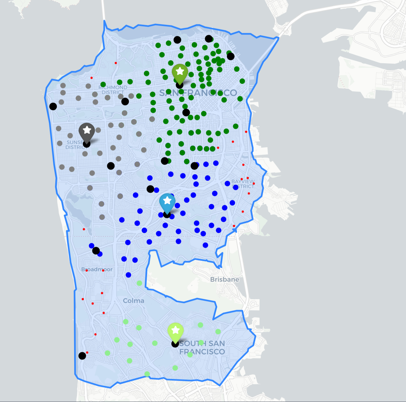
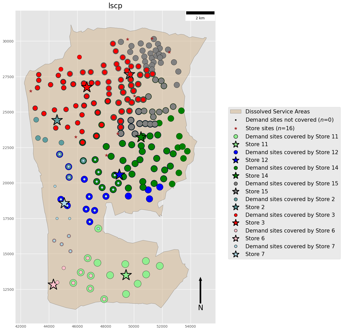
Location Set Covering Problem (LSCP)
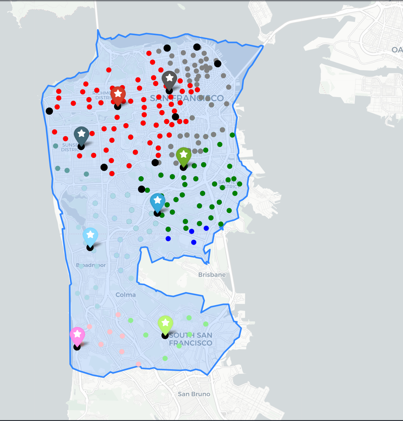
Maximal Coverage Location Problem (MCLP)
MCLP Percentage Covered: 89.7560 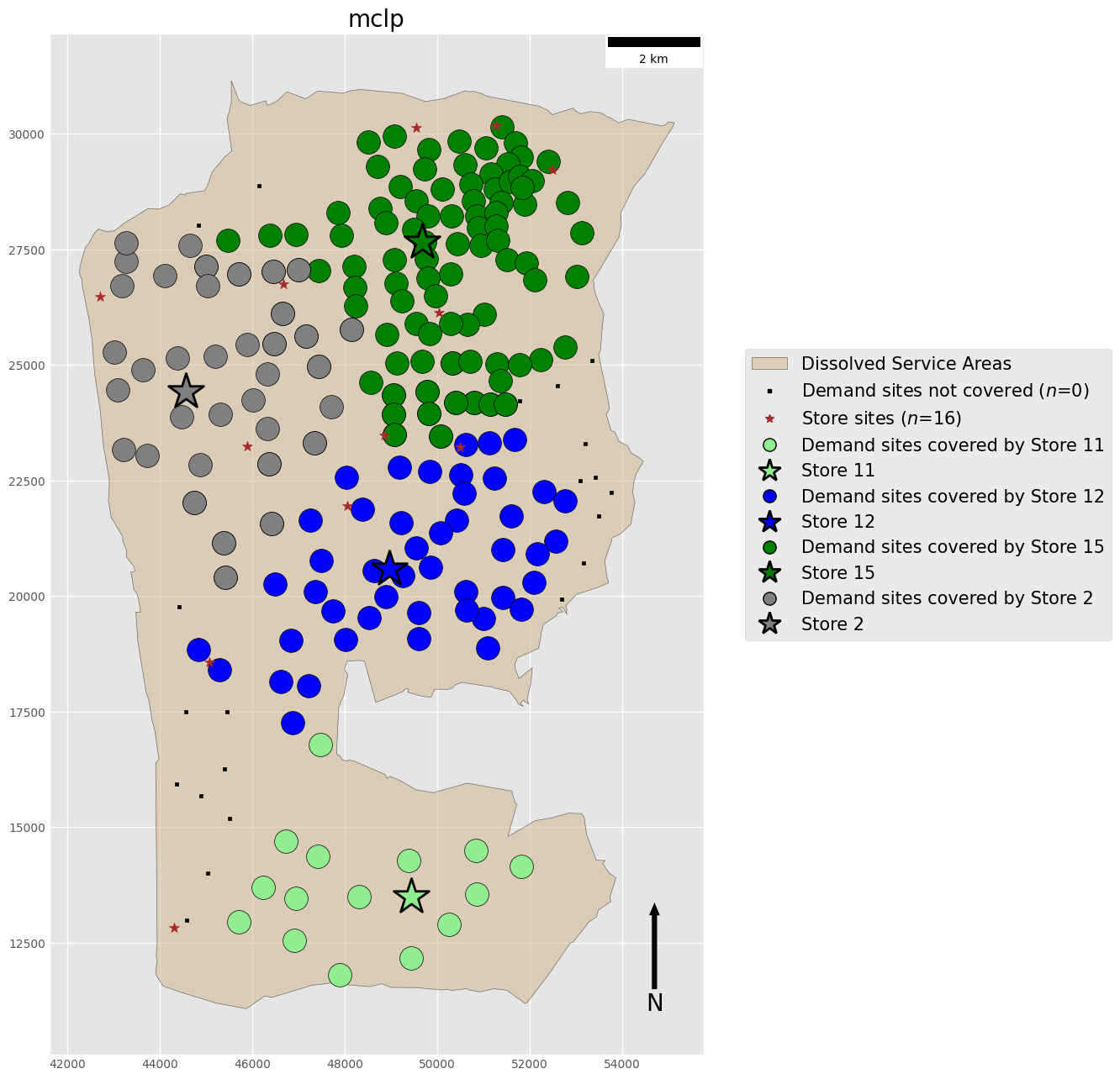
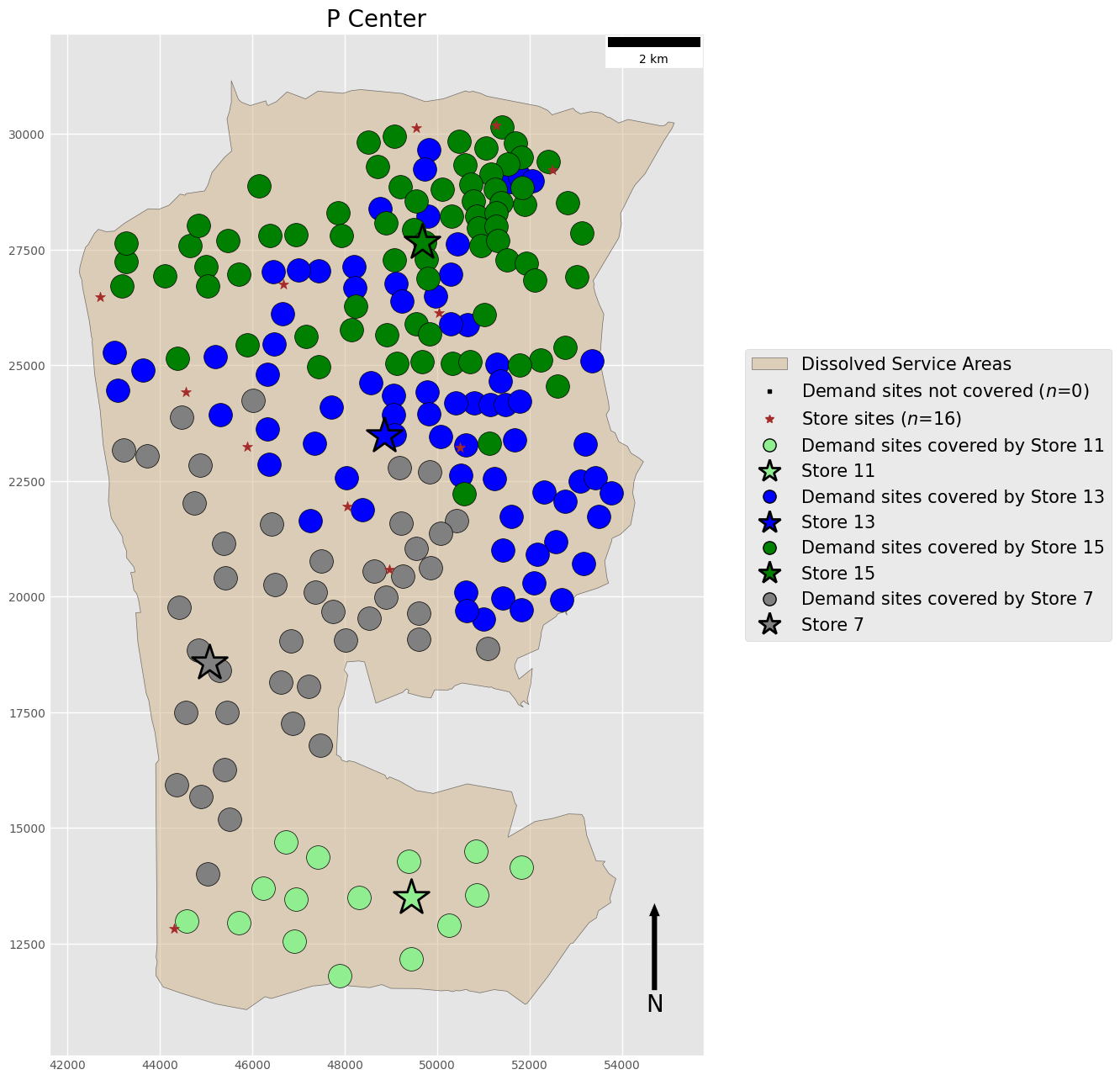
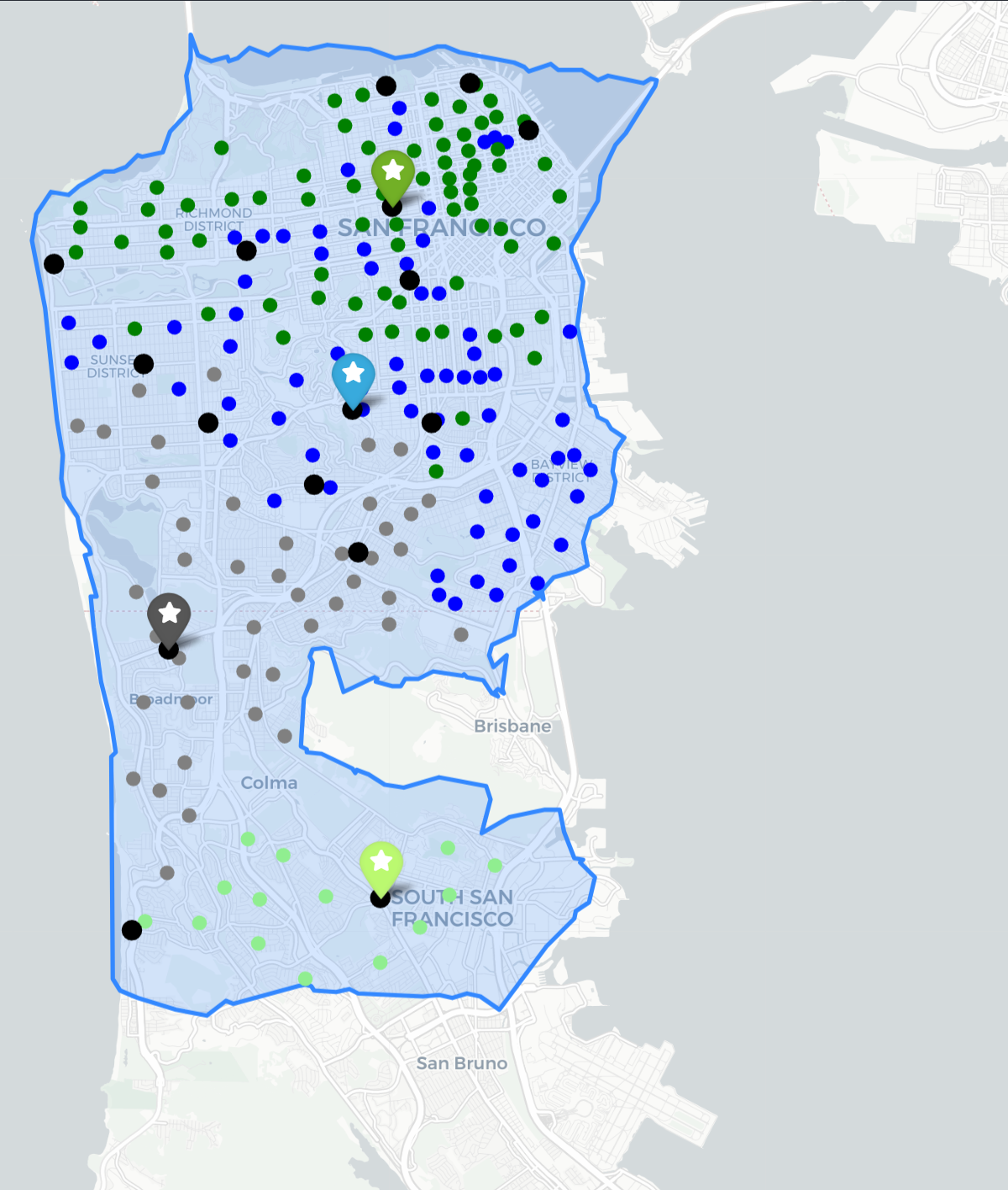
P-Center Problem
problem objective: 7403.06
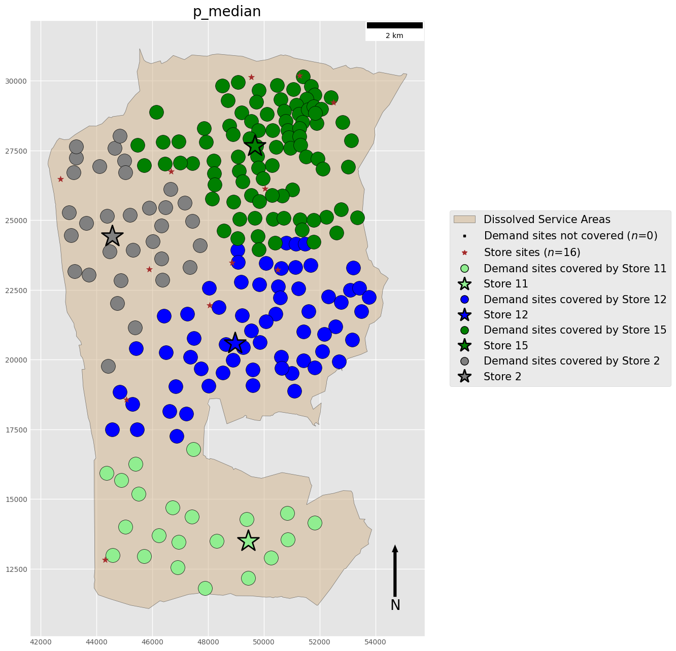
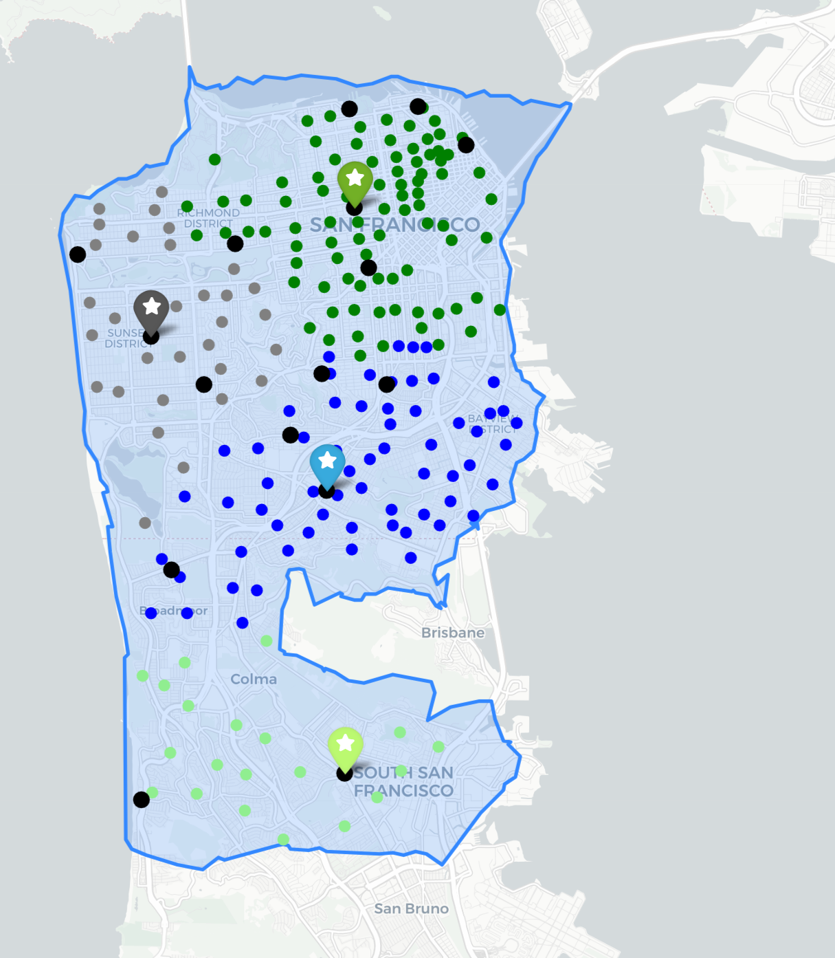
P-Median Problem
p-median mean weighted distance: 2982.1268
problem objective: 2848268129.7145
The plot above clearly demonstrates the key features of each location model:
- LSCP Overlapping clusters of clients associated with multiple facilities All clients covered by at least one facility.
- MCLP Overlapping clusters of clients associated with multiple facilities Potential for complete coverage, but not guranteed.
- p-median Tight and distinct clusters of client-facility relationships All clients allocated to exactly one facility
- p-center Loose and overlapping clusters of client-facility relationships All clients allocated to exactly one facility